Contiguous Sequences

By Michael Kamfonas

Introduction

Let’s say we have a table with sales by product, location and week. We want to enumerate contiguous weeks of sales for each item/location. The table below shows sales for SKU 123 at store A for a range of weeks, and the contiguous week enumeration.

For clarity, we show each fiscal week associated with its end-date. To do this we probably need to join to a Dimension table to translate the FWK_CD to an end-date. Those who use actual dates for time dimension keys would not need this extra join, as the end date would be on the ACTUALS fact. The last column shows the actual enumeration we are seeking to compute. Weeks 2006W19 through 2006W23 all have sales, so they are sequentially enumerated as shown in the last column. Week 2006W24 has no sales, and does not appear in our table. Week 2006W25 is the next week that does, and has to start with sequence number 1 again. Three more consecutive weeks appear, and then there is another gap.

The resulting enumeration can be stored or always derived on the fly to answer questions such as “Find stores that sold SKU 123 for N consecutive weeks during the last year.” The same concept is often used to enumerate weeks out-of-stock. Instead of our table showing weeks that had sales, it shows weeks that the store was out of stock. Various supply-chain or financial methods use such metrics. Here we will only concern ourselves with the technique of enumeration rather than its purpose.

The question is how do we write a SQL query that produces these sequence numbers?

A SQL Solution

One approach is to use a recursive method of traversing consecutive chains of sku/locations over time, and applying the enumeration. This is possible through a procedure, but can also be done with a recursive union, which is now supported by most major database platforms. The problem is that either of these approaches is expensive in resources and very slow. Recursion requires indexed direct access, which is far slower than stream operations that can be pipelined and more effectively parallelized by the DBMS.

Our approach uses the OLAP extension “rank.” We can assume that our set of sales data can be partitioned into many little sets, one for each SKU/STORE. Within each such partition, we will create a rank ordering all rows by time.

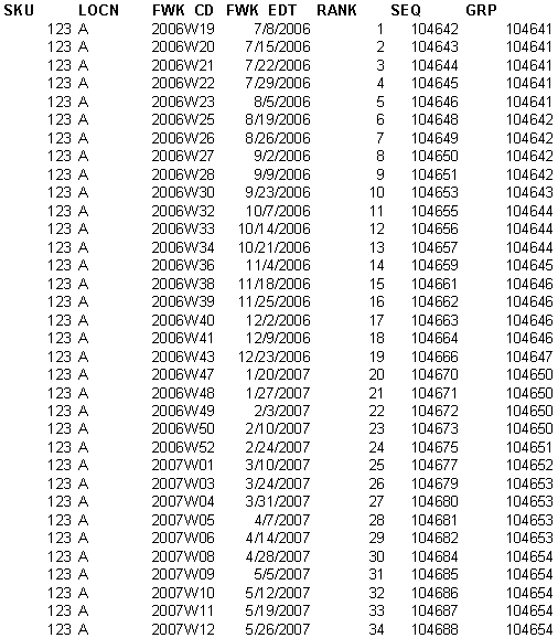
Another useful number we can assign to each row is a sequential number of the week referenced by the row. We can use the DAYS function in DB2, to convert a date to a consecutive number from the beginning of the calendar. Since we are dealing with end-of-week dates, we can divide by 7. The result is an absolute sequence number for each week. The query shown below includes rank and week sequence, as well as their difference, named GRP, which as we will see has particular significance.

Text Box: Select SKU_CD, STORE_CD, A.FWK_CD, FWK_EDT,
rank() over (partition by SKU_CD, STORE_CD order by A.FWK_CD) as RANK,
days(FWK_EDT)/7 SEQ,
days(FWK_EDT)/7 - rank() over (partition by SKU_CD, STORE_CD
order by A.FWK_CD) as GRP
from ACTUALS A join DIM_FWK W on A.FWK_CD=W.FWK_CD

Check the result set shown. The Rank is a sequence number that enumerates all rows within the SKU/LOCN in the order of the fiscal week. The fact that we partitioned by SKU/LOCN causes each SKU/LOCN combination to have its own ranking sequence starting from 1.

If you observe the last column, you will see that contiguous weeks are associated with the same number, and each such group of contiguous weeks has a different value within the SKU/LOCN partition. In other words, each GRP is an identifier of a contiguous-week-set.

In order to get our contiguous numbers, all we have to do is to “rank” each such group in time order. The outcome of this second ranking will be a sequence number starting from 1 for each week within every such group.

Here is the final query…

The result for SKU 123 and LOCN A should be as shown in Table 1.

All examples have been limited to this specific SKU/Location combination. This was done for clarity. The queries produce correct results for all SKUs and Locations.